Documentation

Once the data importation is done, three tabs are visible:

• Raw data: display the imported dataset
• Observations: display the graphics which enable OOT Detection
• Details analysis: display the final mode which is used to define OOT limits.

Each analysis is available for each imported parameter.

 

Raw data tab

The imported dataset is displayed.

Values noted <Limit can be replaced by a numeric value. The replacement value is then used in the statistical analysis.

Fill in the <Limit by cell and click on OK to apply the replacement.

Note: When the replacement value is considered, a note is displayed in the raw data tab (Note: The value of <Limit is ….)

Tip: Values noted “<LOQ” can be replaced by LOQ/2 or LOQ/sqrt(2).

 

Observations tab

View modes

Several viewing modes are available:

• Preview mode: display the simple linear regression for each batch.
• OOT detection: display OOT limits and new batches and highlight OOT results.
• OOT only: subset of the OOT detection mode by focusing on batches with OOT results.
• OOT batch: subset of the OOT detection mode by focusing on OOT batches (if 2 out of 3 consecutive points are detected OOT, the batch is concluded OOT).
• Shelf-life: display for each new batches the estimated shelf-life graph with and without OOT results.

The view mode can be changed by clicking on View Mode in the right window.

Note: By default, the study starts on the preview mode.

Note: If OOT only or/and OOT batch view modes cannot be selected then there is no OOT results or/and no OOT batches in the study.

Note: Direction of change is related to the specifications in dooter (there is no Direction of change field to fill in):

• For a lower ACC, decrease is assumed
• For an upper ACC, decrease is assumed
• For a lower and an upper ACC, unknown is assumed

Batch options

In the left window, the list of the batches is displayed. The color of historical and new batches can be changed.

Note: The replacement color will appear in the report but will not be saved for the future studies. To make the changes permanent see Modify settings section.

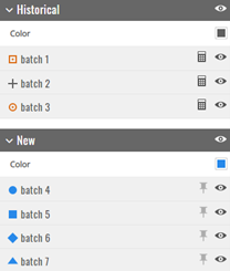
Three icons appear, by clicking on them you can:

	Include/exclude the batch from all analysis (graphs, calculations and analysis are automatically updated)
	Visible/hide the batch in the graphics (the batch is no longer visible on the graphics but is still considered in the calculations), it has no impact on the analysis and enable to switch between modes.
	Switch to shelf-life mode (available only if specification(s) are entered)

 

 

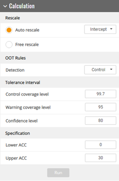
 Statistical options

In the right window statistical option can be changed such as: the rescale value, OOT rules, levels for tolerance intervals and specifications. It allows to customize the analysis at the parameter level.

• The rescale value is set with ‘Auto rescale’ on Intercept (intercept of historical batches) or Average (mean of historical batches at release), or it can be entered by the user with ‘Free rescale’. By default, the rescale is performed on Intercept.
• The OOT Rules: OOT are detected from warning or control limits.
• Tolerance interval
  • Control coverage level: Coverage level for control limits
  • Warning coverage level: coverage level for warning limits
  • Confidence level: Confidence level for control or warning limits
• Specification
  • Lower ACC = Lower Acceptance Criterion/Lower specification
  • Upper ACC = Upper Acceptance Criterion/Upper specification

 

Note: The changes are taken into account in the graphics and the analysis when the icon Run is light grey. If the Run icon is dark grey, the changes are not applied.

Note: The changes will appear in the report but won’t be saved for the future studies. To make the changes permanent see Modify settings section.

 

Graph options

• Graphic options
  • Show or hide the warning limits
  • Highlight or not trace on hover

Note: The changes won’t appear in the report and won’t be saved for the future studies. To make the changes permanent see Modify settings section.

 

Detail analysis tab

The analysis of covariance (i.e. ANCOVA) table is displayed.

The ICH algorithm performed on historical batches is described in the graphics below:

 

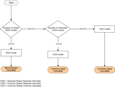
The ANCOVA table details the steps of the algorithm and the final model used to define OOT limits.

A footnote is displayed to explain the final model.

Note: In the situation where there is only one historical batch, the equality of slopes cannot be tested. Then the zero slope is tested.

 

Switch between parameters

There are two ways to switch from on parameter to another:

• with Prev and Next arrows button,
• by clicking on the arrow next to the parameter name and choosing the new parameter.